 | ||||||||||
| Home | Research | Exoplanet Models | Publications | Academic Courses | C.V. | Honors/Awards | My Family | Internal Cultivation | Hobbies | Travels |

| Exoplanet Models |
|
2009~2013:
★A dynamic and interactive tool (Version 5, click HERE to access) to characterize and illustrate the interior structure of exoplanets. In order to run this tool in your web browser, you need to download and install the free Wolfram CDF player.A few important things to note about this tool:
1. The Wolfram CDF Player is completely free and available for download online. You just need to visit www.wolfram.com/cdf-player/ and input your institution's name and any email address to download it.
2. If the tool fails to load in any other web browser, try open it in Firefox.
3. You may need to click "Enable Dynamics" at the upper right-hand corner when necessary to allow the tool to display properly in your web browser.
4. Please be patient, the tool may take a while (up to ~30 seconds) to initialize and load in your web browser. If it runs too slow, try to relaunch your web browser or restart your computer.
5. When you click the Locator, please wait one second before dragging it around, to allow it enough time to respond. DO NOT release the click during the entire dragging process until the Locator is moved to the desired location in the mass-radius diagram.
6. This interactive tool is for research & education purpose only, all rights reserved. If you use this tool, please cite the paper below:
Li Zeng, and Dimitar Sasselov. "A Detailed Model Grid for Solid Planets from 0.1 through 100 Earth Masses". In the Publications of the Astronomical Society of the Pacific (PASP), Chicago Journals, Volume 125, No. 925, pp. 227-239, March 2013. (pdf download)
7. Any questions or comments are much appreciated, please contact me at lzeng@cfa.harvard.eduVersion 5: Important updates: (1) New Planet's M and R and uncertainties (δM+/-, δR+/-) can be plotted as a rectangular uncertainty region with chosen color on the M-R diagram . (2) p0 can be input in GPa. (3) 11 values of p0 range for each Locator {Mass,Radius} are available as 11 clickable buttons. Min and Max values correspond to two-layer planets. (4) Two dashed curves enclose the composition uncertainty in the ternary diagram due to (δM+/-, δR+/-). Please click HERE to access Version 5.Version 4: Important updates: (1) InputField is added to allow users to directly input or change M (Mass in units of Earth Masses) and R (Radius in units of Earth Radii) in numbers, besides clicking and draging the Locator around. After each input, hit Enter or Return on your keyboard to update the calculation. (2) The possible range of central pressure p0 (and Log10[p0]) for a given mass and radius is calculated. Please click HERE to access Version 4.Illustration on how to use it:.jpg) See some older versions below:
Important updates:
(1) Interior density-radius profile and pressure-radius profile are added in.
Please click HERE to access Version 3.
Important updates:
(1) Now the numbers of mass fractions (MF) and outer radii (in R⊕) of every layer are added in.
Please click HERE to access Version 2.
Instruction on how to use Version 2: The three solid black curves correspond to mass-radius relation of three single-layer models (pure-Fe planet, pure-MgSiO3 planet, and pure-H2O planet). The black dot on each of the curve represents the single-layer model at the same central pressure p0. The three single-layer models at p0 are illustrated as red (Fe), green (MgSiO3), and blue (H2O) circles on top to show their relative sizes with respect to each other. For single-layer model, the planet interior structure is uniquely determined by one variable, whether it is central pressure p0, mass M, radius R,... The three dashed curves represent double-layer models. For example, the dashed curve connecting the pure-Fe dot and the pure-H2O dot represents double-layer planet models that consist of a Fe-core and H2O-mantle. Any point on the dashed curve is still at the same central pressure p0, so the dashed curve is an iso-p0 curve. As the point moves along the dashed curve, the central pressure p0 is held as constant while the proportions of Fe and H2O change. For double-layer model, the planet interior structure is uniquely determined by two variables, often its mass M and radius R. For 3-layer model, the planet interior structure is uniquely determined by three variables, so giving its mass M and radius R is not enough, resulting in degeneracy in the solutions. In this case, we choose central pressure p0 as the third variable which can be adjusted and manipulated. Once the central pressure p0 is set, the three dashed curves enclose a triangular region in the mass-radius diagram corresponding to this particular p0. Any point with mass M and radius R which lies within this triangular region can be modeled under this particular p0. In other words, the triangular region represents the phase space in mass-radius diagram which can be achieved by this particular p0. At p0, the tool automatically calculates the mass fractions of the three layers as illustrated in the mass-fraction ternary diagram shown on the left, and it also automatically calculates the relative radii of the three layers as illustrated in the color circle. This tool shows that the mass-fraction ternary diagram is a transformation of the triangular region bounded by dashed curves in the mass-radius diagram. If you press the "Animate" button to increase p0 in steps, you will see that in the mass-radius diagram, the dashed triangular region moves across the point {M,R}with increasing p0 while the point {M,R}is fixed. In the meantime, the red point in the mass-fraction ternary diagram moves along the black curve while the ternary diagram itself is fixed. In the mass-radius diagram, imagine you sit and move together with the dashed triangular region, it is as if the point {M,R}moves across the field of the triangle, producing similar effect as the point in the mass-fraction ternary diagram does.  ★New Interactive Tool Help You Plot Your New Planet on Mass-Radius Diagram: click HERE. (Wolfram CDF Player Required)
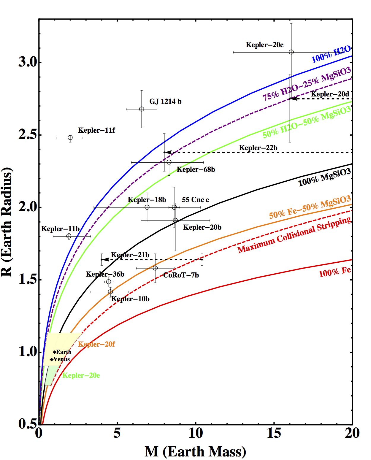
★The following diagram shows the currently known transiting exoplanets with their measured mass and radius with observation uncertainties. Earth and Venus are shown for comparison. The curves are calculated for planets composed of pure Fe, 50% Fe-50% MgSiO3, pure MgSiO3, 50% H2O-50% MgSiO3, 75% H2O-25% MgSiO3 and pure H2O. These percentages are in mass fractions. The data of these six curves are available inTable 1 of paper 1 in Publications. The red dashed curve is the maximum collisional stripping curve calculated by Marcus et al. (2010).
If you use this diagram, please cite the following paper:
Li Zeng, and Dimitar Sasselov. "A Detailed Model Grid for Solid Planets from 0.1 through 100 Earth Masses". In the Publications of the Astronomical Society of the Pacific (PASP), Chicago Journals, Volume 125, No. 925, pp. 227-239, March 2013. (pdf download)
★The following diagram shows the mass-radius contours of double-layer planet. The x-axis is in unit of Earth Masses. The y-axis is in unit of Earth Radii. 1st row: Fe-MgSiO3 planet. 2nd row: MgSiO3-H2O planet. 3rd row: Fe-H2O planet. 1st column: contour mesh of p1/p0 with p0. 2nd column: contour mesh of CMF with p0. 3rd column: contour mesh of CRF with p0.
Given mass and radius input, various sets of mass-radius contours can be used to quickly determine the characteristic interior structure quantities of a 2-layer planet including its p0 (central pressure), p1/p0 (ratio of core-mantle boundary pressure over central pressure), CMF (core mass fraction), and CRF (core radius fraction).The 2-layer model is uniquely solved and represented as a point on the mass-radius diagram given any pair of two parameters from the following list: M (mass), R (radius), p0, p1/p0, CMF, CRF, etc. The contours of constant M or R are trivial on the mass-radius diagram, which are simply vertical or horizontal lines. The contours of constant p0, p1/p0, CMF, or CRF are more useful. Within a pair of parameters, fixing one and continuously varying the other, the point on the mass-radius diagram moves to form a curve. Multiple values of the fixed parameter give multiple parallel curves forming a set of contours. The other set of contours can be obtained by exchanging the fixed parameter for the varying parameter. The two sets of contours crisscross each other to form a mesh, which is a natural coordinate system (see the following figure) of this pair of parameters, superimposed onto the existing Cartesian (M,R) coordinates of the mass-radius diagram. This mesh can be used to determine the two parameters given the mass and radius input or vice versa. 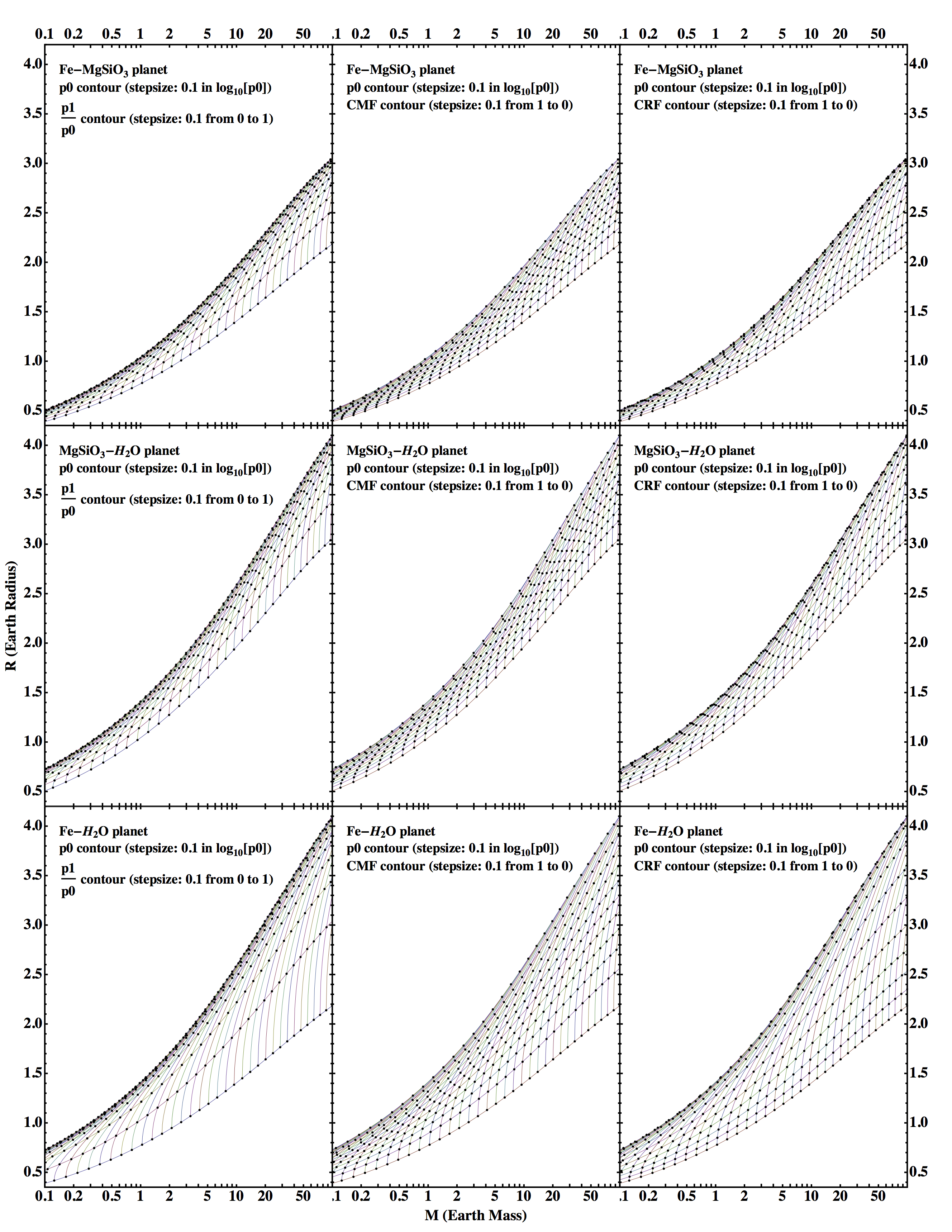
The data for the mass-radius contours with a finer grid are given as follows. Each xls file contains two sheets, one for mass and one for radius, both in Earth units. The rows of the table correspond to Log10[p0] from 8 to 14.4 with stepsize 0.025. The column of the table correspond to one of the three parameters: p1/p0, CMF, or CRF from 0 to 1 in stepsize of 0.025.
This data could be used to transform a probability distribution in mass-radius phase space, into the probability distribution of the interior structure parameter phase space, such as the probability distribution in p0-p1/p0 phase space, p0-CMF phase space, or p0-CRF phase space, assuming double-layer model.
Fe-MgSiO3 planet:
Fe-MgSiO3 p0-CRF tableMgSiO3-H2O planet: MgSiO3-H2O p0-CRF table Fe-H2O planet: Fe-H2O p0-CRF table If you use the diagram or tables, please cite the following paper:
Li Zeng, and Dimitar Sasselov. "A Detailed Model Grid for Solid Planets from 0.1 through 100 Earth Masses". In the Publications of the Astronomical Society of the Pacific (PASP), Chicago Journals, Volume 125, No. 925, pp. 227-239, March 2013. (pdf download)
Summer 2007:
Summer UROP with Prof. Sara Seager on Mass-Radius relation of Earth-like exoplanet.
★We Built Computer Models for the interior structure and the atmosphere of extra-solar planets to understand the Mass-Radius relation and atmospheric spectral lines of exoplanets. Our basic assumption for the interior of Earth-like exoplanets is that they all have an iron core, a silicate mantle and a water crust. We also assumed that the temperature dependence of the Equation Of State (EOS) is negligiable, which is a very good approximation.
Based on these assumptions, we developed two computer codes in matlab to interpret the bulk composition of solid exoplanets based on their mass and radius measurements.
For details, please refer to our paper published on Publications of the Astronomical Society of the Pacific (PASP).
If you use this tool, please cite the following paper:
Li Zeng, and Sara Seager. "A Computational Tool to Interpret the Bulk Composition of Solid Exoplanets based on Mass and Radius Measurements". In the Publications of the Astronomical Society of the Pacific (PASP), Chicago Journals, Volume 120, No. 871, pp. 983-991, September 2008. (pdf download)
Code download instructions:
Frist of all, download the code zip files and decompress them.
Please put the decompressed files into your Matlab work directory so that the Matlab can recognize them. Use addpath command if necessary.
Based in Matlab if using this computer code please cite Li Zeng & Prof. Sara Seager.
ExoterDE(M, Munc, R, Runc); Take a lot of time, but more accurate. This program can deal with the a case of zero uncertainties in planet mass and radius. It plots 1-σ,2-σ,3-σ contours of given Mass, Radius and the uncertainties associated with them.
example: for Mass=10 Earth Mass , Mass uncertainty=0.5 Earth Mass;
Radius= 2 Earth Radius, Radius uncertainty= 0.1 Earth Radius:
just type ExoterDE(10, 0.5, 2, 0.1); in your Matlab command window. Then hit Enter.
ExoterDB(M, Munc, R, Runc); based upon database interpolation. It plots a colormap showing the possible proportions of iron, silicate and water for continuous range of σ from 0 up to 3.
example: for Mass=10 Earth Mass , Mass uncertainty=0.5 Earth Mass;
Radius= 2 Earth Radius, Radius uncertainty= 0.1 Earth Radius:
just type ExoterDB(10, 0.5, 2, 0.1); in your Matlab command window. Then hit Enter.
The results should look similar to the diagram below:
.png) |
 | |
No comments:
Post a Comment